Recursion and recursive algorithms. Recursion and recursive algorithms Given a recursive algorithm procedure f n integer
A presentation on the topic “Recursive Algorithms” was created to prepare students for the Unified State Exam in computer science and ICT. The paper examines the definition of recursion and provides examples of recursively defined graphical objects. The presentation contains methods for solving task No. 11 from the draft demo version of the Unified State Exam - 2015 in computer science. The first method involves building a call tree, the second method solves the problem using the substitution method. 4 examples of solving problems using both methods are considered. The following presentation contains 25 exercises for training with answers from Konstantin Polyakov’s website.
Download:
Preview:
To use presentation previews, create an account for yourself ( account) Google and log in: https://accounts.google.com
Slide captions:
Task No. 11 Unified State Exam (basic level, time - 5 minutes) Recursive algorithms. Author – Korotun O.V., computer science teacher, Municipal Educational Institution “Secondary School No. 71”
What you need to know: Recursion is in the definition, description, depiction of an object or process within this object or process itself, that is, a situation when an object is part of itself. Coat of arms Russian Federation is a recursively defined graphic object: in the right paw of the double-headed eagle depicted on it, a scepter is clamped, which is crowned with a reduced copy of the coat of arms. Since on this coat of arms there is also a scepter in the right paw of the eagle, an infinite recursion is obtained. Recursive coat of arms of Russia
In programming, recursion is a call to a function from itself, directly or through other functions, for example, function A calls function B, and function B calls function A. The number of nested calls to a function or procedure is called the depth of recursion. example of recursion: If you have a grease stain on your dress, don't worry. Oil stains are removed with gasoline. Gasoline stains are removed with an alkali solution. The alkali is removed with essence. Rub the trace of the essence with oil. Well, you already know how to remove oil stains!
Example assignment: Given a recursive algorithm: procedure F(n: integer); begin writeln(n); if n
Example assignment: Given a recursive algorithm: procedure F(n: integer); begin writeln(n) ; if n
Example assignment: Given a recursive algorithm: procedure F(n: integer); begin writeln(n); if n Slide 9
Example assignment: Given a recursive algorithm: procedure F(n: integer); begin writeln(n); if n Slide 10
Example assignment: Given a recursive algorithm: procedure F(n: integer); begin writeln(n); if n Slide 11
15 Example No. 2: A recursive algorithm is given: procedure F(n: integer); begin writeln(n); if n
Example No. 2: Given a recursive algorithm: procedure F(n: integer); begin writeln(n); if n Slide 13
Example No. 3: Given a recursive algorithm: procedure F(n: integer); begin writeln("*") ; if n > 0 then begin F(n-2); F(n div 2) end end ; How many asterisks will be printed on the screen when calling F(7)? 7 5 3 2 3 1 1 1 1 In this example, the symbol * -2 div 2 1 0 -1 0 -1 0 -1 -1 -1 0 0 0 is displayed on the screen rather than the values of the parameter n .
Example No. 3: Given a recursive algorithm: procedure F(n: integer); begin writeln("*"); if n > 0 then begin F(n-2); F(n div 2) end end ; How many asterisks will be printed on the screen when calling F(7)? * By counting the number of “stars”, we get 21 In this example, it is not the values of the parameter n that are displayed on the screen, but the symbol * * * * * * * * * * * * * * * * * * * * * *
Example No. 3: Given a recursive algorithm: procedure F(n: integer); begin writeln("*"); if n > 0 then begin F(n-2); F(n div 2) end end ; How many asterisks will be printed on the screen when calling F(7)? Let's solve the problem without a tree. Let S(n) be the number of “stars” that will be printed when calling F(n). Then 1+S(n-2)+ S(n div 2), n>0 1 , n We need to know S(7). S(7)= 1 +S(5)+ S(3) S(5)= 1 +S(3)+S(2) S(3)= 1 +S(1)+S(1) S( 2)=1+S(0)+S(1)=1+1+S(1)=2+S(1) S(1)= 1+ S(-1)+S(0)=1+ 1+1=3 Reverse: S(2)=2+3=5 S(3)=1+3+3=7 S(5)=1+7+5=13 S(7)=1+ 13+7= 21 S(n)=
Example No. 4: procedure F(n: integer); begin if n Slide 18
Example No. 4: procedure F(n: integer); begin if n Slide 19
Example No. 4: procedure F(n: integer); begin if n
Example No. 4: procedure F(n: integer); begin if n
Training tasks
Problem 1: Given a recursive algorithm: procedure F(n: integer); begin writeln("*"); if n > 0 then begin F(n-2); F(n div 2); F(n div 2); end end ; How many asterisks will be printed on the screen when calling F(5)? Answer: 34
Problem 2: Given a recursive algorithm: procedure F(n: integer); begin writeln("*"); if n > 0 then begin F(n-2); F(n-2); F(n div 2); end end ; How many asterisks will be printed on the screen when calling F(6)? Answer: 58
Problem 3: Given a recursive algorithm: procedure F(n: integer); begin writeln("*"); if n > 0 then begin F(n-3); F(n div 2); end end ; How many asterisks will be printed on the screen when calling F(7)? Answer: 15
Problem 4: Given a recursive algorithm: procedure F(n: integer); begin writeln("*"); if n > 0 then begin F(n-3); F(n-2); F(n div 2); end end ; How many asterisks will be printed on the screen when calling F(7)? Answer: 55
Problem 5: Given a recursive algorithm: procedure F(n: integer); begin writeln("*"); if n > 0 then begin F(n-3); F(n-2); F(n div 2); F(n div 2); end end ; How many asterisks will be printed on the screen when calling F(6)? Answer: 97
Problem 6: Given a recursive algorithm: procedure F(n: integer); begin writeln("*"); if n > 0 then begin writeln("*"); F(n-2); F(n div 2); end end ; How many asterisks will be printed on the screen when calling F(7)? Answer: 31
Problem 7: Given a recursive algorithm: procedure F(n: integer); begin writeln("*"); if n > 0 then begin writeln("*"); F(n-2); F(n div 2); F(n div 2); end end; How many asterisks will be printed on the screen when calling F(7)? Answer: 81
Problem 8: Given a recursive algorithm: procedure F(n: integer); begin writeln("*"); if n > 0 then begin writeln("*"); F(n-2); F(n-2); F(n div 2); end end; How many asterisks will be printed on the screen when calling F(6)? Answer: 77
Problem 9: Given a recursive algorithm: procedure F(n: integer); begin if n > 0 then begin F(n-2); F(n-1); F(n-1); end; writeln("*"); end ; How many asterisks will be printed on the screen when calling F(5)? Answer: 148
Problem 10: Given a recursive algorithm: procedure F(n: integer); begin if n > 0 then begin writeln("*"); F(n-2); F(n-1); F(n-1); end; writeln("*"); end; How many asterisks will be printed on the screen when calling F(5)? Answer: 197
Problem 11: Given a recursive algorithm: procedure F(n: integer); begin if n > 1 then begin F(n-2); F(n-1); F(n div 2); end; writeln("*"); end ; How many asterisks will be printed on the screen when calling F(7)? Answer: 88
Problem 12: Given a recursive algorithm: procedure F(n: integer); begin if n > 2 then begin writeln("*"); F(n-2); F(n-1); F(n div 2); end ; writeln("*"); end; How many asterisks will be printed on the screen when calling F(6)? Answer: 33
Problem 13: Given a recursive algorithm: procedure F (n: integer); begin writeln(n); if n
Problem 14: Given a recursive algorithm: procedure F (n: integer); begin writeln(n); if n
Problem 15: Given a recursive algorithm: procedure F (n: integer); begin writeln(n); if n
Problem 16: Given a recursive algorithm: procedure F (n: integer); begin writeln(n); if n
Problem 17: Given a recursive algorithm: procedure F (n: integer); begin writeln(n); if n
Problem 18: Given a recursive algorithm: procedure F (n: integer); begin writeln(n); if n
Problem 19: Given a recursive algorithm: procedure F (n: integer); begin writeln(n); if n
Problem 20: Given a recursive algorithm: procedure F (n: integer); begin writeln(n); if n
Problem 21: Given a recursive algorithm: procedure F (n: integer); begin writeln(n); if n
Problem 22: Given a recursive algorithm: procedure F (n: integer); begin writeln(n); if n
Problem 23: Given a recursive algorithm: procedure F (n: integer); begin writeln(n); if n
Problem 24: Given a recursive algorithm: procedure F (n: integer); begin writeln(n); if n
Problem 25: Given a recursive algorithm: procedure F (n: integer); begin writeln(n); if n
Recursion is when a subroutine calls itself. When faced with such an algorithmic design for the first time, most people experience certain difficulties, but with a little practice, recursion will become an understandable and very useful tool in your programming arsenal.
1. The essence of recursion
A procedure or function may contain calls to other procedures or functions. The procedure can also call itself. There is no paradox here - the computer only sequentially executes the commands it encounters in the program and, if it encounters a procedure call, it simply begins to execute this procedure. It doesn't matter what procedure gave the command to do this.
Example of a recursive procedure:
Procedure Rec(a: integer); begin if a>
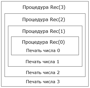
Let's consider what happens if a call, for example, of the form Rec(3) is made in the main program. Below is a flowchart showing the execution sequence of the statements.
Rice. 1. Block diagram of the recursive procedure.
Procedure Rec is called with parameter a = 3. It contains a call to procedure Rec with parameter a = 2. The previous call has not completed yet, so you can imagine that another procedure is created and the first one does not finish its work until it finishes. The calling process ends when parameter a = 0. At this point, 4 instances of the procedure are executed simultaneously. The number of simultaneously performed procedures is called recursion depth.
The fourth procedure called (Rec(0)) will print the number 0 and finish its work. After this, control returns to the procedure that called it (Rec(1)) and the number 1 is printed. And so on until all procedures are completed. The original call will print four numbers: 0, 1, 2, 3.
Another visual image of what is happening is shown in Fig. 2.
Rice. 2. Executing the Rec procedure with parameter 3 consists of executing the Rec procedure with parameter 2 and printing the number 3. In turn, executing the Rec procedure with parameter 2 consists of executing the Rec procedure with parameter 1 and printing the number 2. Etc.
As an exercise on your own, consider what happens when you call Rec(4). Also consider what would happen if you called the Rec2(4) procedure below, with the operators reversed.
Procedure Rec2(a: integer); begin writeln(a); if a>0 then Rec2(a-1); end;
Please note that in these examples the recursive call is inside a conditional statement. This necessary condition in order for the recursion to ever end. Also note that the procedure calls itself with a different parameter than the one with which it was called. If the procedure does not use global variables, then this is also necessary so that the recursion does not continue indefinitely.
A slightly more complex scheme is possible: function A calls function B, which in turn calls A. This is called complex recursion. It turns out that the procedure described first must call a procedure that has not yet been described. For this to be possible, you need to use .
Procedure A(n: integer); (Forward description (header) of the first procedure) procedure B(n: integer); (Forward description of the second procedure) procedure A(n: integer); (Full description of procedure A) begin writeln(n); B(n-1); end; procedure B(n: integer); (Full description of procedure B) begin writeln(n); if n
The forward declaration of procedure B allows it to be called from procedure A. The forward declaration of procedure A is not required in this example and is added for aesthetic reasons.
If ordinary recursion can be likened to an ouroboros (Fig. 3), then the image of complex recursion can be drawn from the famous children's poem, where “The wolves were frightened and ate each other.” Imagine two wolves eating each other and you will understand complex recursion.

Rice. 3. Ouroboros - a snake devouring its own tail. Drawing from the alchemical treatise “Synosius” by Theodore Pelecanos (1478).

Rice. 4. Complex recursion.
3. Simulating a loop using recursion
If a procedure calls itself, it essentially causes the instructions it contains to be executed again, similar to a loop. Some programming languages do not contain looping constructs at all, leaving programmers to organize repetitions using recursion (for example, Prolog, where recursion is a basic programming technique).
For example, let's simulate the operation of a for loop. To do this, we need a step counter variable, which can be implemented, for example, as a procedure parameter.
Example 1.
Procedure LoopImitation(i, n: integer); (The first parameter is the step counter, the second parameter is the total number of steps) begin writeln("Hello N ", i); //Here are any instructions that will be repeated if i The result of a call of the form LoopImitation(1, 10) will be the execution of instructions ten times, changing the counter from 1 to 10. In this case, the following will be printed: Hello N 1 In general, it is not difficult to see that the parameters of the procedure are the limits for changing the counter values. You can swap the recursive call and the instructions to be repeated, as in the following example. Example 2.
Procedure LoopImitation2(i, n: integer); begin if i In this case, a recursive procedure call will occur before instructions begin to be executed. The new instance of the procedure will also, first of all, call another instance, and so on, until we reach the maximum value of the counter. Only after this the last of the called procedures will execute its instructions, then the second to last one will execute its instructions, etc. The result of calling LoopImitation2(1, 10) will be to print greetings in reverse order: Hello N 10 If we imagine a chain of recursively called procedures, then in example 1 we go through it from earlier called procedures to later ones. In example 2, on the contrary, from later to earlier. Finally, a recursive call can be placed between two blocks of instructions. For example: Procedure LoopImitation3(i, n: integer); begin writeln("Hello N ", i); (The first block of instructions may be located here) if i Here, the instructions from the first block are first executed sequentially, then the instructions from the second block are executed in reverse order. When calling LoopImitation3(1, 10) we get: Hello N 1 It would take two loops to do the same thing without recursion. You can take advantage of the fact that the execution of parts of the same procedure is spaced out over time. For example: Example 3: Converting a number to binary.
Obtaining the digits of a binary number, as is known, occurs by dividing with a remainder by the base of the number system 2. If there is a number, then its last digit in its binary representation is equal to Taking the whole part of division by 2: we get a number that has the same binary representation, but without the last digit. Thus, it is enough to repeat the above two operations until the next division field receives an integer part equal to 0. Without recursion it will look like this: While x>0 do begin c:=x mod 2; x:=x div 2; write(c); end; The problem here is that the digits of the binary representation are calculated in reverse order (latest first). To print a number in normal form, you will have to remember all the numbers in the array elements and print them in a separate loop. Using recursion, it is not difficult to achieve output in the correct order without an array and a second loop. Namely: Procedure BinaryRepresentation(x: integer); var c, x: integer; begin (First block. Executed in order of procedure calls) c:= x mod 2; x:= x div 2; (Recursive call) if x>0 then BinaryRepresentation(x); (Second block. Executed in reverse order) write(c); end; Generally speaking, we did not receive any winnings. The digits of the binary representation are stored in local variables, which are different for each running instance of the recursive procedure. That is, it was not possible to save memory. On the contrary, we waste extra memory storing many local variables x. However, this solution seems beautiful to me. A sequence of vectors is said to be given by a recurrence relation if the initial vector and the functional dependence of the subsequent vector on the previous one are given A simple example of a quantity calculated using recurrence relations is the factorial The next factorial can be calculated from the previous one as: By introducing the notation , we obtain the relation: The vectors from formula (1) can be interpreted as sets of variable values. Then the calculation of the required element of the sequence will consist of repeated updating of their values. In particular for factorial: X:= 1; for i:= 2 to n do x:= x * i; writeln(x); Each such update (x:= x * i) is called iteration, and the process of repeating iterations is iteration. Let us note, however, that relation (1) is a purely recursive definition of the sequence and the calculation of the nth element is actually the repeated taking of the function f from itself: In particular, for factorial one can write: Function Factorial(n: integer): integer; begin if n > 1 then Factorial:= n * Factorial(n-1) else Factorial:= 1; end; It should be understood that calling functions entails some additional overhead, so the first option for calculating the factorial will be slightly faster. In general, iterative solutions work faster than recursive ones. Before moving on to situations where recursion is useful, let's look at one more example where it should not be used. Let's consider special case recurrent relationships, when the next value in a sequence depends not on one, but on several previous values at once. An example is the famous Fibonacci sequence, in which each next element is the sum of the previous two: With a “frontal” approach, you can write: Function Fib(n: integer): integer; begin if n > 1 then Fib:= Fib(n-1) + Fib(n-2) else Fib:= 1; end; Each Fib call creates two copies of itself, each copy creates two more, and so on. The number of operations increases with the number n exponentially, although for an iterative solution linear in n number of operations. In fact, the above example teaches us not WHEN recursion should not be used, otherwise HOW it should not be used. After all, if there is a fast iterative (loop-based) solution, then the same loop can be implemented using a recursive procedure or function. For example: // x1, x2 – initial conditions (1, 1) // n – number of the required Fibonacci number function Fib(x1, x2, n: integer): integer; var x3: integer; begin if n > 1 then begin x3:= x2 + x1; x1:= x2; x2:= x3; Fib:= Fib(x1, x2, n-1); end else Fib:= x2; end; Still, iterative solutions are preferable. The question is, when in this case should you use recursion? Any recursive procedures and functions that contain just one recursive call to themselves can be easily replaced by iterative loops. To get something that doesn't have a simple non-recursive counterpart, you need to resort to procedures and functions that call themselves two or more times. In this case, the set of called procedures no longer forms a chain, as in Fig. 1, but a whole tree. There are wide classes of problems when the computational process must be organized in this way. For them, recursion will be the simplest and most natural solution. The theoretical basis for recursive functions that call themselves more than once is the section discrete mathematics studying trees. Definition:
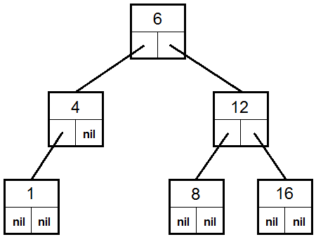
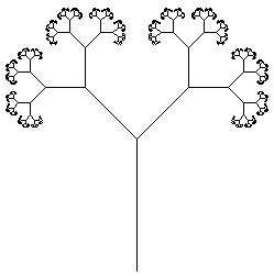
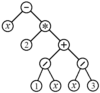
we will call the finite set T, consisting of one or more nodes such that: This definition is recursive. In short, a tree is a set consisting of a root and subtrees attached to it, which are also trees. A tree is defined through itself. However this definition makes sense, since the recursion is finite. Each subtree contains fewer nodes than its containing tree. In the end, we come to subtrees containing only one node, and this is already clear what it is. Rice. 3. Tree. In Fig. Figure 3 shows a tree with seven nodes. Although ordinary trees grow from bottom to top, it is customary to draw them the other way around. When drawing a diagram by hand, this method is obviously more convenient. Because of this inconsistency, confusion sometimes arises when one node is said to be above or below another. For this reason, it is more convenient to use the terminology used when describing family trees, calling nodes closer to the root ancestors, and more distant ones descendants. Graphically, a tree can be depicted in some other ways. Some of them are shown in Fig. 4. According to the definition, a tree is a system of nested sets, where these sets either do not intersect or are completely contained in one another. Such sets can be depicted as regions on a plane (Fig. 4a). In Fig. 4b, the nested sets are not located on a plane, but are elongated into one line. Rice. 4b can also be viewed as a diagram of some algebraic formula containing nested parentheses. Rice. Figure 4c gives another popular way of representing a tree structure as a staggered list. Rice. 4. Other ways to depict tree structures: (a) nested sets; (b) nested parentheses; (c) concession list. The staggered list has obvious similarities to the way program code is formatted. Indeed, a program written within the framework of the structured programming paradigm can be represented as a tree consisting of nested structures. You can also draw an analogy between a ledge list and appearance tables of contents in books where sections contain subsections, which in turn contain subsections, etc. The traditional way of numbering such sections (section 1, subsections 1.1 and 1.2, subsection 1.1.2, etc.) is called the Dewey decimal system. Applied to the tree in Fig. 3 and 4 this system will give: 1. A; 1.1B; 1.2 C; 1.2.1 D; 1.2.2 E; 1.2.3 F; 1.2.3.1 G; In all algorithms related to tree structures, the same idea invariably appears, namely the idea passing or tree traversal. This is a way of visiting tree nodes in which each node is traversed exactly once. This results in a linear arrangement of tree nodes. In particular, there are three ways: you can go through the nodes in forward, reverse and end order. Forward traversal algorithm: This algorithm is recursive, since the traversal of a tree contains the traversal of subtrees, and they, in turn, are traversed using the same algorithm. In particular, for the tree in Fig. 3 and 4, direct traversal gives a sequence of nodes: A, B, C, D, E, F, G. The resulting sequence corresponds to a left-to-right enumeration of nodes when representing a tree using nested parentheses and in Dewey decimal notation, as well as a top-down passage when representing it as a staggered list. When implementing this algorithm in a programming language, hitting the root corresponds to the procedure or function performing some actions, and going through subtrees corresponds to recursive calls to itself. In particular, for a binary tree (where each node has at most two subtrees), the corresponding procedure would look like this: // Preorder Traversal – English name for direct order procedure PreorderTraversal((Arguments)); begin //Passing the root DoSomething((Arguments)); //Transition of the left subtree if (There is a left subtree) then PreorderTransversal((Arguments 2)); //Transition of the right subtree if (There is a right subtree) then PreorderTransversal((Arguments 3)); end; That is, first the procedure performs all actions, and only then all recursive calls occur. Reverse traversal algorithm: That is, all subtrees are traversed from left to right, and the return to the root is located between these traversals. For the tree in Fig. 3 and 4 this gives the sequence of nodes: B, A, D, C, E, G, F. In a corresponding recursive procedure, the actions will be located in the spaces between the recursive calls. Specifically for a binary tree: // Inorder Traversal – English name for reverse order procedure InorderTraversal((Arguments)); begin //Traveling the left subtree if (There is a left subtree) then InorderTraversal((Arguments 2)); //Passing the root DoSomething((Arguments)); //Traversal of the right subtree if (There is a right subtree) then InorderTraversal((Arguments 3)); end; End-order traversal algorithm: For the tree in Fig. 3 and 4 this will give the sequence of nodes: B, D, E, G, F, C, A. In a corresponding recursive procedure, the actions will be located after the recursive calls. Specifically for a binary tree: // Postorder Traversal – English name for the end order procedure PostorderTraversal((Arguments)); begin //Traveling the left subtree if (There is a left subtree) then PostorderTraversal((Arguments 2)); //Transcending the right subtree if (There is a right subtree) then PostorderTraversal((Arguments 3)); //Passing the root DoSomething((Arguments)); end; If some information is located in tree nodes, then an appropriate dynamic data structure can be used to store it. In Pascal, this is done using a record type variable containing pointers to subtrees of the same type. For example, a binary tree where each node contains an integer can be stored using a variable of type PTree, which is described below: Type PTree = ^TTree; TTree = record Inf: integer; LeftSubTree, RightSubTree: PTree; end; Each node has a PTree type. This is a pointer, meaning each node must be created by calling the New procedure on it. If the node is a leaf node, then its LeftSubTree and RightSubTree fields are assigned the value nil. Otherwise, the LeftSubTree and RightSubTree nodes are also created by the New procedure. One such record is shown schematically in Fig. 5. Rice. 5. Schematic representation of a TTree type record. The record has three fields: Inf – a number, LeftSubTree and RightSubTree – pointers to records of the same TTree type. An example of a tree made up of such records is shown in Figure 6. Rice. 6. A tree made up of TTree type records. Each entry stores a number and two pointers that can contain either nil, or addresses of other records of the same type. If you have not previously worked with structures consisting of records containing links to records of the same type, we recommend that you familiarize yourself with the material about. Let's consider the algorithm for drawing the tree shown in Fig. 6. If each line is considered a node, then this image fully satisfies the definition of a tree given in the previous section. Rice. 6. Tree. The recursive procedure would obviously draw one line (the trunk up to the first branch), and then call itself to draw the two subtrees. Subtrees differ from the tree containing them in the coordinates of their starting point, rotation angle, trunk length, and the number of branches they contain (one less). All these differences should be made parameters of the recursive procedure. An example of such a procedure, written in Delphi, is presented below: Procedure Tree(Canvas: TCanvas; //Canvas on which the tree will be drawn x,y: extended; //Root coordinates Angle: extended; //Angle at which the tree grows TrunkLength: extended; //Trunk length n: integer / /Number of branches (how many more //recursive calls remain)); var x2, y2: extended; //Trunk end (branch point) begin x2:= x + TrunkLength * cos(Angle); y2:= y - TrunkLength * sin(Angle); Canvas.MoveTo(round(x), round(y)); Canvas.LineTo(round(x2), round(y2)); if n > 1 then begin Tree(Canvas, x2, y2, Angle+Pi/4, 0.55*TrunkLength, n-1); Tree(Canvas, x2, y2, Angle-Pi/4, 0.55*TrunkLength, n-1); end; end; To obtain Fig. 6 this procedure was called with the following parameters: Tree(Image1.Canvas, 175, 325, Pi/2, 120, 15); Note that drawing is carried out before recursive calls, that is, the tree is drawn in direct order. According to legend in the Great Temple of Banaras, under the cathedral marking the middle of the world, there is a bronze disk on which 3 diamond rods are fixed, one cubit high and thick as a bee. A long time ago, at the very beginning of time, the monks of this monastery committed offense before the god Brahma. Enraged, Brahma erected three high rods and placed 64 pure gold discs on one of them, so that each smaller disc rested on a larger one. As soon as all 64 disks are transferred from the rod on which God Brahma placed them when creating the world, to another rod, the tower along with the temple will turn into dust and the world will perish under thunderclaps. Independently of Brahma, this puzzle was proposed at the end of the 19th century by the French mathematician Edouard Lucas. The sold version usually used 7-8 disks (Fig. 7). Rice. 7. Puzzle “Towers of Hanoi”. Let's assume that there is a solution for n-1 disk. Then for shifting n disks, proceed as follows: 1) Shift n-1 disk. Because for the case n= 1 the rearrangement algorithm is obvious, then by induction, using actions (1) – (3), we can rearrange an arbitrary number of disks. Let's create a recursive procedure that prints the entire sequence of rearrangements for a given number of disks. Each time such a procedure is called, it must print information about one shift (from point 2 of the algorithm). For rearrangements from points (1) and (3), the procedure will call itself with the number of disks reduced by one. //n – number of disks //a, b, c – pin numbers. Shifting is done from pin a, //to pin b with auxiliary pin c. procedure Hanoi(n, a, b, c: integer); begin if n > 1 then begin Hanoi(n-1, a, c, b); writeln(a, " -> ", b); Hanoi(n-1, c, b, a); end else writeln(a, " -> ", b); end; Note that the set of recursively called procedures in this case forms a tree traversed in reverse order. The task of parsing is to calculate the value of the expression using an existing string containing an arithmetic expression and the known values of the variables included in it. The process of calculating arithmetic expressions can be represented as a binary tree. Indeed, each of the arithmetic operators (+, –, *, /) requires two operands, which will also be arithmetic expressions and, accordingly, can be considered as subtrees. Rice. Figure 8 shows an example of a tree corresponding to the expression: Rice. 8. Syntax tree corresponding to the arithmetic expression (6). In such a tree, the end nodes will always be variables (here x) or numeric constants, and all internal nodes will contain arithmetic operators. To execute an operator, you must first evaluate its operands. Thus, the tree in the figure should be traversed in terminal order. Corresponding sequence of nodes called reverse Polish notation arithmetic expression. When building a syntax tree, you should pay attention to next feature. If, for example, there is an expression and we will read the operations of addition and subtraction from left to right, then the correct syntax tree will contain a minus instead of a plus (Fig. 9a). In fact, this tree corresponds to the expression. It is possible to make the creation of a tree easier if you analyze expression (8) in reverse, from right to left. In this case, the result is a tree with Fig. 9b, equivalent to tree 8a, but not requiring replacement of signs. Similarly, from right to left, you need to analyze expressions containing multiplication and division operators. Rice. 9. Syntax trees for expression a – b + c when reading from left to right (a) and from right to left (b). This approach does not completely eliminate recursion. However, it allows you to limit yourself to only one call to the recursive procedure, which may be sufficient if the motive is to maximize performance. The idea of this approach is to replace recursive calls with a simple loop that will be executed as many times as there are nodes in the tree formed by the recursive procedures. What exactly will be done at each step should be determined by the step number. Comparing the step number and the necessary actions is not a trivial task and in each case it will have to be solved separately. For example, let's say you want to do k nested loops n steps in each: For i1:= 0 to n-1 do for i2:= 0 to n-1 do for i3:= 0 to n-1 do … If k is unknown in advance, it is impossible to write them explicitly, as shown above. Using the technique demonstrated in Section 6.5, you can obtain the required number of nested loops using a recursive procedure: Procedure NestedCycles(Indexes: array of integer; n, k, depth: integer); var i: integer; begin if depth To get rid of recursion and reduce everything to one cycle, note that if you number the steps in the radix number system n, then each step has a number consisting of the numbers i1, i2, i3, ... or the corresponding values from the Indexes array. That is, the numbers correspond to the values of the cycle counters. Step number in regular decimal notation: There will be a total of steps n k. By going through their numbers in the decimal number system and converting each of them to the radix system n, we get the index values: M:= round(IntPower(n, k)); for i:= 0 to M-1 do begin Number:= i; for p:= 0 to k-1 do begin Indexes := Number mod n; Number:= Number div n; end; DoSomething(Indexes); end; Let us note once again that the method is not universal and you will have to come up with something different for each task. 1. Determine what the following recursive procedures and functions will do. (a) What will the following procedure print when Rec(4) is called? Procedure Rec(a: integer); begin writeln(a); if a>0 then Rec(a-1); writeln(a); end; (b) What will be the value of the function Nod(78, 26)? Function Nod(a, b: integer): integer; begin if a > b then Nod:= Nod(a – b, b) else if b > a then Nod:= Nod(a, b – a) else Nod:= a; end; (c) What will be printed by the procedures below when A(1) is called? Procedure A(n: integer); procedure B(n: integer); procedure A(n: integer); begin writeln(n); B(n-1); end; procedure B(n: integer); begin writeln(n); if n (d) What will the procedure below print when calling BT(0, 1, 3)? Procedure BT(x: real; D, MaxD: integer); begin if D = MaxD then writeln(x) else begin BT(x – 1, D + 1, MaxD); BT(x + 1, D + 1, MaxD); end; end; 2. Ouroboros - a snake devouring its own tail (Fig. 14) when unfolded has a length L, diameter around the head D, abdominal wall thickness d. Determine how much tail he can squeeze into himself and how many layers will the tail be laid in after that? Rice. 14. Expanded ouroboros. 3. For the tree in Fig. 10a indicate the sequence of visiting nodes in forward, reverse and end traversal order. 4. Graphically depict the tree defined using nested brackets: (A(B(C, D), E), F, G). 5. Graphically depict the syntax tree for the following arithmetic expression: Write this expression in reverse Polish notation. 6. For the graph below (Fig. 15), write down the adjacency matrix and the incidence matrix. 1. Having calculated the factorial sufficiently large number times (a million or more), compare the effectiveness of recursive and iterative algorithms. How much will the execution time differ and how will this ratio depend on the number whose factorial is being calculated? 2. Write a recursive function that checks the correct placement of parentheses in a string. If the arrangement is correct, the following conditions are met: (a) the number of opening and closing parentheses is equal. Examples of incorrect placement:)(, ())(, ())((), etc. 3. The line may contain both round and square brackets. Each opening bracket has a corresponding closing bracket of the same type (round - round, square - square). Write a recursive function that checks whether the parentheses are placed correctly in this case. Example of incorrect placement: ([) ]. 4. The number of regular bracket structures of length 6 is 5: ()()(), (())(), ()(()), ((())), (()()). Note: Correct parenthesis structure of minimum length "()". Structures of longer length are obtained from structures of shorter length in two ways: (a) if the smaller structure is taken into brackets, 5. Create a procedure that prints all possible permutations for integers from 1 to N. 6. Create a procedure that prints all subsets of the set (1, 2, ..., N). 7. Create a procedure that prints all possible representations of the natural number N as the sum of other natural numbers. 8. Create a function that calculates the sum of the array elements using the following algorithm: the array is divided in half, the sums of the elements in each half are calculated and added. The sum of the elements in half the array is calculated using the same algorithm, that is, again by dividing in half. Divisions occur until the resulting pieces of the array contain one element each and calculating the sum, accordingly, becomes trivial. Comment: This algorithm is an alternative. In the case of real-valued arrays, it usually allows for smaller rounding errors. 10. Create a procedure that draws the Koch curve (Figure 12). 11. Reproduce the figure. 16. In the figure, at each subsequent iteration the circle is 2.5 times smaller (this coefficient can be made a parameter). 1. D. Knuth. The art of computer programming. v. 1. (section 2.3. “Trees”).
Hello N 2
…
Hello N 10
…
Hello N 1
…
Hello N 10
Hello N 10
…
Hello N 14. Recurrence relations. Recursion and Iteration
5. Trees
5.1. Basic definitions. Ways to depict trees
a) There is one special node called the root of this tree.
b) The remaining nodes (excluding the root) are contained in pairwise disjoint subsets, each of which in turn is a tree. Trees are called subtrees of this tree.

5.2. Passing trees
5.3. Representation of a tree in computer memory

6. Examples of recursive algorithms
6.1. Drawing a tree
6.2. Hanoi Towers
The process requires that the larger disk never end up on top of the smaller one. The monks are in a quandary: in what order should they do the shifts? It is required to provide them with software to calculate this sequence.
2) Shift n th disk onto the remaining free pin.
3) We shift the stack from n-1 disk received in point (1) on top n-th disk.6.3. Parsing arithmetic expressions

7.3. Determining a tree node by its number
Security questions

Tasks
(b) within any pair there is an opening - corresponding closing bracket, the brackets are placed correctly.
Write a recursive program to generate all regular bracket structures of length 2 n.
(b) if two smaller structures are written sequentially.
Literature
2. N. Wirth. Algorithms and data structures.